This article is Part I of a set of five technical articles that accompany a whitepaper written in collaboration between Meta and Ekimetrics. Object Detection (OD) and Optical Character Recognition (OCR) were used to detect specific features in creative images, such as faces, smiles, text, brand logos, etc. Then, in combination with impressions data, marketing mix models were used to investigate what objects, or combinations of objects in creative images in marketing campaigns, drive higher ROIs. In this Part I we explore the methodology for using pre-trained Detectron2 models to detect brand-specific object in creative images.
Why you should read this
Manual labeling of the Training and Validation data sets
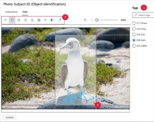
Figure 1 - Microsoft Azure Machine Learning Studio Image labeling Tool. Source: Microsoft.
Distribution of Objects in Manually labeled Data set and Implications for the labeling of the Unlabeled Data set
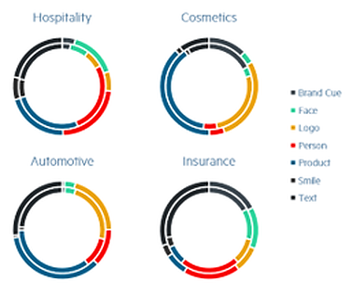
Figure 2 - The distribution of labeled objects in the Train (outer) and Validation (inner) data sets.
Models
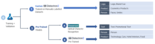
Figure 3 - Object Detection using different pre-trained and custom-trained models.
Pre-Trained Models
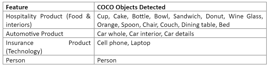
Figure 4 - COCO Objects Detected in Pre-Trained Models, Present in Creatives of Brands Studied
Choosing a Detectron2 Pre-Trained Model
The performance on Accuracy and Confidence Score (see figure 5 - Definition Box 1) were compared for three models :
Model 1: Faster R-CNN R50 FPN 1x
Model 2: Faster R-CNN R101 FPN 3x
Model 3: Faster R-CNN X 101 32x8d FPN 3x
Overall, Model 3 has the highest average Accuracy while Model 2 has the highest average Confidence Score. The number of creatives with correctly identified objects is highest in Model 3. Figure 6 shows the results.
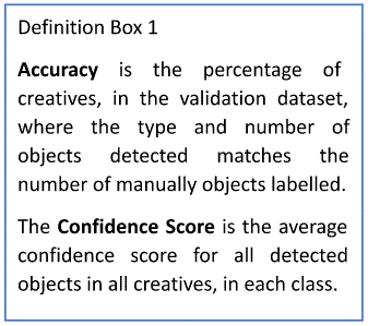
Figure 5 - Definition Box 1
More in detail, for each object type:
- People: All three models have varying performance in detecting people across different brands. Overall, Model 3 has the highest accuracy.
- Technology: Model 2 is most confident in detecting tech, but misses tech in many creatives entirely. Overall, Model 3 has the highest accuracy.
- Cars: Model 3 has the highest average confidence and accuracy in detecting cars.
- Hotel Interiors and Food: Model 2 and Model 3 have a similar performance in detecting food and interior, both higher than Model 1.
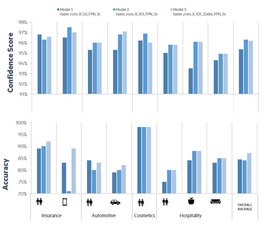
Figure 6 - Comparison in performance on the validation data set of three pre-trained Detectron2 models.
Figures 7 and 8 show the performance of Model 3 on the specific Objects of interest. In particular, the Confidence Scores (figure 8) that lead to the high Accuracies in figure 7 range from between 80% to 98%. As we developed our methodology to be applicable regardless of the industry, we needed to choose a Confidence Score Threshold of Acceptance that is high enough to ensure accuracy, but not too high that it would miss objects of interest entirely. Therefore, a threshold of 85% confidence was selected.

Figure 7 - Accuracy of Faster R-CNN X 101 32x8d FPN 3x on Specific Object Types.

Figure 8 - Average Confidence of Faster R-CNN X 101 32x8d FPN 3x on Specific Object Types.
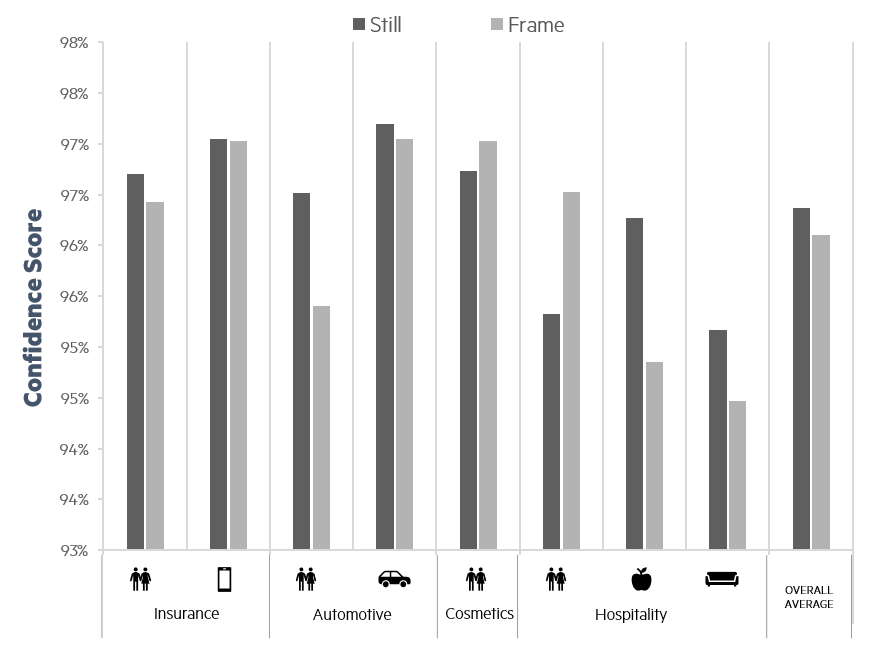
Figure 9 - Performance of Faster R-CNN X 101 32x8d FPN 3x on Still vs Frame images.
Useful links
Snippets of code
Installations
!pip install detectron2 -f https://dl.fbaipublicfiles.com/detectron2/wheels/$CUDA_VERSION/torch$TORCH_VERSION/index.html
Import libraries
import detectron2
from detectron2.engine import DefaultPredictor
from detectron2.config import get_cfg
from detectron2.data import MetadataCatalog, data setCatalog
from detectron2.utils.visualizer import ColorMode, Visualizer
from detectron2 import model_zoo
from detectron2.evaluation import COCOEvaluator, inference_on_data set
from detectron2.data import build_detection_test_loader

from PIL import Image
import cv2
Define detector class
class Detector:

    def __init__(self):
        self.cfg = get_cfg()

        # Load model config and pretrained model
        model_name = "COCO-Detection/faster_rcnn_R_101_FPN_3x.yaml"
#         model_name = "COCO-Detection/faster_rcnn_R_50_FPN_1x.yaml"
#         model_name = "COCO-Detection/faster_rcnn_X_101_32x8d_FPN_3x.yaml"
        self.cfg.merge_from_file(model_zoo.get_config_file(model_name))
        self.cfg.MODEL.WEIGHTS = model_zoo.get_checkpoint_url(model_name)

        self.cfg.MODEL.ROI_HEADS.SCORE_THRESH_TEST = 0.85
        self.cfg.MODEL.DEVICE = "cpu" # or cuda

        self.predictor = DefaultPredictor(self.cfg)

    # Define a function to visualise the result of the prediction on an image and print the label IDs
    def onImages(self, imagePath, if_visualise=False, if_print=False):

        # Get predictions
        image = cv2.imread(imagePath)
        predictions = self.predictor(image)

        instances = predictions["instances"]
        class_indexes = instances.pred_classes
        prediction_boxes = instances.pred_boxes

        class_catalog = MetadataCatalog.get(self.cfg.data setS.TRAIN[0]).thing_classes
        class_labels = [class_catalog[i] for i in class_indexes]

        class_scores = instances.scores


        # Visualise preditions
        if if_visualise:
            viz = Visualizer(image[:,:,::-1],
                               metadata = MetadataCatalog.get(self.cfg.data setS.TRAIN[0]),
                               #scale=1
                               instance_mode = ColorMode.IMAGE_BW #IMAGE #SEGMENTATION #IMAGE_BW
                              )
            output = viz.draw_instance_predictions(predictions["instances"].to("cpu"))
            plt.figure(figsize = (25,17))
            plt.imshow(output.get_image()[:, :, ::-1])

        # Print labels
        if if_print:
            print(f"Class Labels: {class_labels}")
            print(f"Class Confidence Scores: {class_scores}")
            print(f"Class Indexes: {class_indexes}")
            print(f"Prediction Boxes: {prediction_boxes}")


        return class_indexes, prediction_boxes, class_labels, class_scores


    # valuate its performance using AP metric implemented in COCO API.
    # https://detectron2.readthedocs.io/modules/evaluation.html#detectron2.evaluation.COCOEvaluator

    def evaluate(self, data set_name):

        evaluator = COCOEvaluator(data set_name, self.cfg.OUTPUT_DIR)#self.cfg, False, self.cfg.OUTPUT_DIR)
        val_loader = build_detection_test_loader(self.cfg, data set_name)
        result = inference_on_data set(self.predictor.model, val_loader, evaluator)
        print(result)
Run detector
# label new creatives
job_name = 'new_creatives_set_50_scores_faster_rcnn_X_101_32x8d_FPN_3x'
datapath = "your-data-path"
save_path = "your-save-path"

# get list of all image files to process
im_files_ext = ['jpg','png','jpeg','gif','webp','tiff','psd','raw','bmp','heif','indd','jpeg 2000','svg','ai','eps','pdf']
ims_list = []
for ext in im_files_ext:
    temp = glob.glob(f'{datapath}*.{ext}')
    for file in temp:
        ims_list.append(file)

num_files = len(ims_list)
print(num_files)
print(ims_list)

# Initialise detector
detector = Detector()


# Run detector on chunks
j = 1 # for keeping track of chunk

for chunk in chunks:

    # Create export file
    df = pd.DataFrame(columns=['file_name', ' class_indexes', 'prediction_boxes', 'class_labels', 'class_scores'])

    i = 1 # for keeping track of file number

    for im_file in chunk:
        start = time.time()
        class_indexes, prediction_boxes, class_labels, class_scores = detector.onImages(f'{im_file}', if_visualise=False, if_print=False)
        new_row = {'file_name': im_file,
                   'class_indexes': class_indexes.tolist(),
                   'prediction_boxes': prediction_boxes,
                   'class_labels': class_labels,
                   'class_scores': class_scores.tolist()
                  }
        df = df.append(new_row, ignore_index=True)
        end = time.time()

        print(f'\tChunk {j}/{len(chunks)} - file {i}/{len(chunk)}: {im_file} took {end-start} seconds.')
        i = i + 1

    sp = f'{save_path}{job_name}_chunk_{j}.csv'
    df.to_csv(sp, sep=',', header=True, index=False)
    print(f"\t\tJSON saved in: {sp}")
    j = j + 1
Other helpful code
def display_im_path(dbfs_img_path, figsize=(14,10)):

    image = Image.open(dbfs_img_path)
    plt.figure(figsize=(14,10))
    plt.imshow(image)
    plt.axis('off')
    plt.show()
def display_im_array(array, figsize=(14,10)):

    plt.figure(figsize=figsize)
    plt.imshow(array)
    plt.axis('off')
    plt.show()
def get_files(basepath, num=None):

    all_files = os.listdir(basepath)
    im_files_ext = ['jpg','png','jpeg','gif','webp','tiff','psd','raw','bmp','heif','indd','jpeg 2000','svg','ai','eps','pdf']
    img_list_all = [f"{basepath}{file}" for file in all_files if file.split('.')[-1] in im_files_ext]

#     random.shuffle(img_list_all)
    if num:
        return img_list_all[:num]
    else:
        return img_list_all
Next article
After having explored Detector2 pre-trained models in this first part, in the next article, we will present custom-trained Detectron2 models, how they were used to detect logos, brand cues, faces and smiles, and code snipped on how to optimise parameter values. Stay tuned!
Appendix
Resources
Detectron2
For both the pre-trained and custom models, a Faster R-CNN algorithm was used due to its speed and high performance on small object detection. This algorithm combines two network models: Fast R-CNN (Region based Convolutional Neural Network), a deep learning algorithm which generates a convolutional feature map, and RPN (Regi on Proposal Networks), a convolutional network that proposes regions.
The specific model used was Faster R-CNN X 101 32x8d FPN 3x, a Faster R-CNN model developed by Detectron2 which uses a FPN (Feature Pyramid Networks) backbone, and a learning rate schedule of 3x. This model was chosen based on the baseline performances reported by FAIR, which highlight this model as having the highest average precision and training memory. For more information. Furthermore, the model was tested and evaluated against the performance of other Faster R-CNN models on objects the models are pre-trained on, against out Validation set. Figure 6 shows the results.
Manipulating Bounding Boxes
In order to train the Custom-Trained Models, the Azure format was converted to the Detectron2 format: COCO bounding box (bbox) is defined as [x_min, y_min, width, height].
JSON files exported from Azure Data labeling have bounding boxes that are normalised. Detectron2 expect the bounding boxes in absolute values. Therefore, we transformed the attribute 'bbox' of the COCO file downloaded from Azure ML Studio to denormalise it, and added the 'bbox_mode' attribute to be equal to 1 (XYWH_ABS 0). We also add the pair "iscrowd:0" to each annotation [8].
In order to limit the region in images for text detection to outside of Logo and Product objects, Detectron2 format was transformed to Tesseract format: Detectron2 format [X, Y, W, H] to the Tesseract format (x1=X, x2=W+X, y1=Y, y2=H+Y).
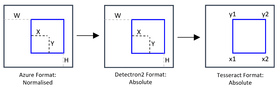
Figure 10 - Manipulation of bounding boxes to accommodate each technology. The first transformation (from left to right) was necessary to train Custom-Trained models. The second transformation was necessary to limit the region in images for text detection to anything outside of logo or product objects.
Detecting Faces with Open libraries with Pre-Trained Models
To detect Faces and Smiles, we began by exploring open libraries that have pre-trained models for this purpose. Figure 11 shows some of the libraries available, as well as those we tested.
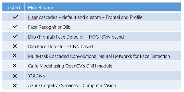
Figure 11 - Open libraries with pre-trained models that detect faces and smiles, and those we tested.

Figure 12 - Smiles being detected inside faces only was a necessary methodology we implemented, to improve the accuracy of open libraries that detect faces and smiles.
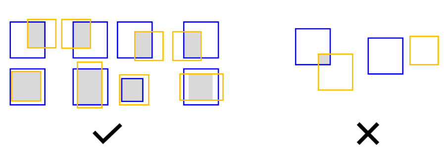
Figure 13 - Methodology for assessing whether a predicted label for Face or Smile is accurate. Blue boxes indicate the bounding box of manually labeled objects. Yellow boxes indicate those for predicted objects. The grey area indicates the Region of Intersection (ROI). If the grey areas are between 60% and 130% of the size of the manually labeled object’s bounding box, the predicted label was considered to be accurate.