Exploring the links between creative execution and marketing effectiveness - Part II Custom trained Detectron2 for OD

This article is Part II of a set of five technical articles that accompany a whitepaper written in collaboration between Meta and Ekimetrics. Object Detection (OD) and Optical Character Recognition (OCR) were used to detect specific features in creative images, such as faces, smiles, text, brand logos, etc. Then, in combination with impressions data, marketing mix models were used to investigate what objects, or combinations of objects in creative images in marketing campaigns, drive higher ROIs. In this Part II we explore the methodology for training Detectron2 models to detect brand-specific object in creative images.

Why you should read this

This article is mostly directed to machine learning practitioners. Here you will find a practical application of object detection algorithms; we present different open-source resources, comparisons and trade-offs in model selection for specific objects, methodology to improve performance for custom datasets, and how the object detection is then used to make inferences on the impact of creatives in marketing strategies.

Dataset

Our dataset contained >50k image and video creatives across four different brands. The main goal of the custom object detection (OD) was to detect three types of brand-specific objects - logo, product and brand cue - as well as faces and smiles. Initially, faces and smiles were detected by pre-trained algorithms such as Haar cascades and Dlib, but due to the poor performance, it was decided to use a custom algorithm.

Before beginning the OD process, videos were converted to images by extracting every tenth frame. Training and Validation sets were then created using the Microsoft Azure Machine Learning Studio labelling tool. The labels were then converted to COCO format, and registered in Detectron as custom COCO libraries. Read more about this in Part I.

## Registering COCO format datasets
from detectron2.data.datasets import register_coco_instances

register_coco_instances(train, {'thing_classes': train_metadata.thing_classes, 'thing_dataset_id_to_contiguous_id': train_metadata.thing_dataset_id_to_contiguous_id}, train_json_path, TRAINING_IMAGES_PATH)
register_coco_instances(valid, {'thing_classes': valid_metadata.thing_classes, 'thing_dataset_id_to_contiguous_id': valid_metadata.thing_dataset_id_to_contiguous_id}, valid_json_path, VALID_IMAGES_PATH)

Algorithm

The Faster Region-based Convolutional Neural Network (R-CNN) model, Faster R-CNN X 101 32x8d FPN 3x, was used for the custom OD model.

One model was trained per object per brand using the manually labelled training sets. For detecting faces and smiles, the training set consisted of creatives from all four brands, but each model was developed separately for face and smile per brand. In total there were, thus, 19 custom models. The validation set was used to tune hyperparameters of each model, with accuracy as the main metric. The final models were then used to detect objects in the unlabelled images for all four brands. The training, validation and final detections were all done using a single node GPU (CUDA) on Databricks.

Hyperparameter Tuning

Process

While Detectron2 allows for the customization of many configurations, including learning rate, backbone, image size, and number of images per batch, we limited the scope to just three parameters due to time constraints. These are summarized in Table 1 along with the parameter values tested. The choice of parameters was based on those deemed to be the most influential in performance. In addition to these parameters, the learning rate – the rate at which the algorithm converges to a solution – was customized. Rather than using the default value of 0.001, the learning rate was determined by the linear learning rate scaling rule. This was done in order to facilitate training on larger batch sizes.

 

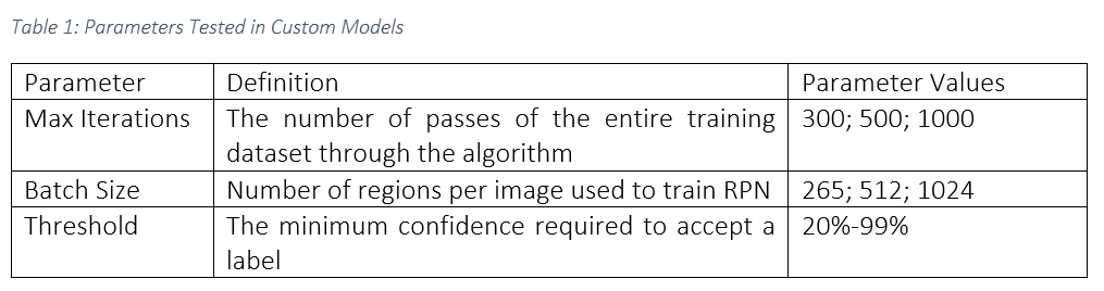
Table 1: Parameters Tested in Custom Models

Example Code

## Parameters values to test
parameters = {
    'SOLVER.MAX_ITER': [300, 500, 1000],
    'ROI_HEADS.BATCH_SIZE_PER_IMAGE': [265, 512, 1024]
}

## Configuring the algorithmn
def config_detectron(train_dataset, max_iter, batchsize):
    classes = MetadataCatalog.get(train_dataset).thing_classes
    num_classes = len(classes)
    print(f"Number of classes in dataset: {num_classes}")
    cfg = get_cfg()
    cfg.merge_from_file(model_zoo.get_config_file("COCO-Detection/faster_rcnn_X_101_32x8d_FPN_3x.yaml"))
    cfg.DATASETS.TRAIN = (train_dataset, )
    cfg.DATASETS.TEST = ()
    cfg.DATALOADER.NUM_WORKERS = 0
    cfg.MODEL.WEIGHTS = model_zoo.get_checkpoint_url("COCO-Detection/faster_rcnn_X_101_32x8d_FPN_3x.yaml") # Let training initialize from model zoo
    cfg.SOLVER.IMS_PER_BATCH = 2 ## # How many images per batch? The original models were trained on 8 GPUs with 16 images per batch, since we have 1 GPUs: 16/8 = 2 (we actually have 2 GPUs but we cannot use both as we do not have enough CUDA memory)
    cfg.SOLVER.BASE_LR = 0.00125 # We do the same calculation with the learning rate as the GPUs, the original model used 0.01, so we'll divide by 8: 0.01/8 = 0.00125. 
    cfg.SOLVER.MAX_ITER = max_iter   # How many iterations are we going for? 
    cfg.MODEL.ROI_HEADS.BATCH_SIZE_PER_IMAGE = batchsize
    cfg.MODEL.ROI_HEADS.NUM_CLASSES = num_classes
    os.makedirs(cfg.OUTPUT_DIR, exist_ok=True)
    print(dbutils.fs.ls(cfg.OUTPUT_DIR))
    return cfg

### Training
def train_detectron(config):
    trainer = DefaultTrainer(config)
    trainer.resume_or_load(resume=False)
    trainer.train()
    return trainer

Exhaustive Grid Search was used to determine the combination of Max Iterations and Batch Size that yielded the highest accuracy on the validation set for each model. The results were visualized on a heat map, with confidence thresholds of 20%, 40%, 60%, and 80%. An example is shown in Figure 1. In this example, the model with Max Iteration of 1000 and a Batch Size of 265 performed the best, and the results did not improve beyond a confidence threshold of 40%. Confusion Matrices (see example in Figure 2) were also used to gain insight into the False Positive vs. False Negative rate.

 

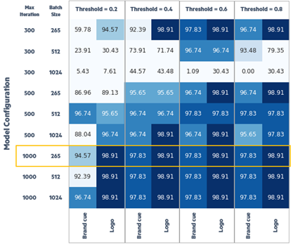
Figure 1 : Example Results of Grid Search

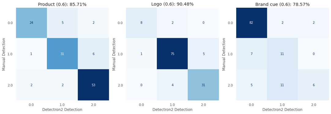
Figure 2 : Example Confusion Matrices for Best Performing Model with 80% Confidence Threshold

## Prediction
def prediction(config, test_dataset, date_string, threshold):
    cfg = config
    cfg.MODEL.WEIGHTS = f'/dbfs/mnt/trd/{brand}/objectdetection/custom_output/GPU/{date_string}/model_final.pth'
    cfg.MODEL.ROI_HEADS.SCORE_THRESH_TEST = threshold # set the testing threshold for this model
    cfg.DATASETS.TEST = (test_dataset, )
    predictor = DefaultPredictor(cfg)
    return predictor

def evaluation(config, test_dataset, trainer):
    # Setup an evaluator, we use COCO because it's one of the standards for object detection: https://detectron2.readthedocs.io/modules/evaluation.html#detectron2.evaluation.COCOEvaluator
    evaluator = COCOEvaluator(dataset_name=test_dataset, 
                              cfg=config, 
                              distributed=False, 
                              output_dir="./output/")

    # Create a dataloader to load in the test data (cmaker-fireplace-valid)
    val_loader = build_detection_test_loader(config, 
                                             dataset_name=test_dataset)

    # Make inference on the validation dataset: https://detectron2.readthedocs.io/tutorials/evaluation.html
    inference = inference_on_dataset(model=trainer, # get the model from the trainer
                         data_loader=val_loader, 
                         evaluator=evaluator)
    return inference

## Make Predictions
def get_predictions(predictor, imagePath):
        
    # Get predictions
    image = cv2.imread(imagePath)
    predictions = predictor(image)

    instances = predictions["instances"]
    class_indexes = instances.pred_classes
    prediction_boxes = instances.pred_boxes

    class_catalog = valid_metadata.thing_classes
    class_labels = [class_catalog[i] for i in class_indexes] 

    class_scores = instances.scores

    return class_indexes, prediction_boxes, class_labels, class_scores

Results

The best performing model was then used to determine the optimal threshold for each object type, at 1% intervals ranging from 20% to 99%. The threshold yielding the highest accuracy for each object class per model was then selected. The results are summarized in Table 2. Following these results, the best custom-trained model per object per brand was used to detect object in the unlabelled dataset in batches of 200 creatives. This was done in order to limit the CUDA memory and ensure that work was saved along the way should something happen. The total detection time for each brand ranged between 72-168 hours.

 

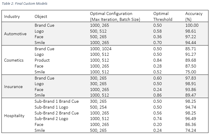
Table 2: Final Custom Models

Useful links

• Detectron2 - Github
• Detectron2 - Documentation
• Detectron2 - ModelZoo

Other useful code

Imports

# Install Detectron2 dependencies: https://detectron2.readthedocs.io/tutorials/install.html (use cu100 because colab is on CUDA 10.0)
!pip install -U torch==1.4+cu100 torchvision==0.5+cu100 -f https://download.pytorch.org/whl/torch_stable.html 
!pip install cython pyyaml==5.1
!pip install -U 'git+https://github.com/cocodataset/cocoapi.git#subdirectory=PythonAPI'

!pip install awscli # you'll need this if you want to download images from Open Images (we'll see this later)

# Make sure we can import PyTorch (what Detectron2 is built with)
import torch, torchvision
torch.__version__
!gcc --version
!pip install detectron2 -f https://dl.fbaipublicfiles.com/detectron2/wheels/cu100/index.html

# Setup detectron2 logger
import detectron2
from detectron2.utils.logger import setup_logger
setup_logger() # this logs Detectron2 information such as what the model is doing when it's training# import some common detectron2 utilities

# Other detectron2 imports
from detectron2.engine import DefaultTrainer
from detectron2.evaluation import COCOEvaluator, inference_on_dataset
from detectron2.data import build_detection_test_loader
from detectron2 import model_zoo 
from detectron2.engine import DefaultPredictor 
from detectron2.config import get_cfg
from detectron2.utils.visualizer import Visualizer 
from detectron2.data import MetadataCatalog 

Next article

In the next article, we will showcase Tesseract, a open-source optical character recognition (OCR) Engine, and the image-processing methods we developed to raise the baseline performance of this library, from 68% accuracy, by up to 28 percentage points.