
Summary
We propose to illustrate how far BERT-type models can be considered as interpretable by design. We show that the attention coefficients specific to BERT architecture constitute a particularly rich piece of information that can be used to perform interpretability. There are mainly two ways to do interpretability: attribution and generation of counterfactual examples. Here we propose to evaluate how attention coefficients can form the basis of an attribution method. We will show in a second article how they can also be used to set up counterfactuals.
The BERT architecture
An artificial neural network is a computer system inspired by the functioning of the human brain and biological neurons to learn specific tasks. The neural networks represent a subset of machine learning algorithms. In order to perform a learning task, the neural network spreads information through an elementary network, called a perceptron. The way in which information is diffused can be formalized through linear algebra and the manipulation of various activation functions. A neural network can be defined as an association of elementary objects called formal neurons, like the perceptron. There are several types of layers that can be part of a neural network:
- Fully connected layers, which receive a vector as input, and produce a new vector as output by applying a linear combination and possibly an activation function;
- Convolution layers, which learn localized patterns in space;
- Attention layers, which model the general relations between different objects.
Attention mechanisms are particularly effective for natural language processing tasks. This is mainly due to the fact that they allow to properly model a word through mathematical representations. In particular, attention layers make it possible to assign a contextual representation of the word on a case-by-case basis. This makes it a much more efficient tool than Word2vec since the latter only models an average context, but does not adapt to the given situation. Attention mechanisms are at the heart of Transformers-type models as shown in the diagram below. The BERT model corresponds to a stack of the left part of the generic architecture of a Transformer [1].
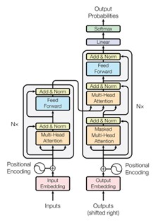
Figure 1 - Transformers architecture
Fine tuning of BERT for sentiment analysis
To illustrate how attention coefficients can be a source of interpretability in natural language processing, we propose to fine tune a DistilBERT for sentiment analysis. A DistilBERT is a distilled version of BERT. It is smaller, faster, cheaper, lighter and recovers 97% of BERT’s performance on GLUE [2]. A perfect compromise, in fact. Most transformers are available pre-trained on the Hugging Face transformers library [3]. The objective is to perform supervised classification on the IMDB database to assess the sentiment associated with a movie review. An illustration of the dataset is shown below:
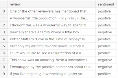
Figure 2 - IMDB sample
To do so, we import all the libraries needed. In particular, the tokenizer DistilBertTokenizer and the pre-trained hugging face model TFDistilBertForSequenceClassification are used.
tokenizer = DistilBertTokenizer.from_pretrained('distilbert-base-uncased')
sentence_encoder = TFDistilBertForSequenceClassification.from_pretrained('distilbert-base-uncased', output_attentions = True)
The parameter "output_attention" must be equal to "True". It will allow us to retrieve the attention coefficients of the model. We add a dense layer with a softmax activation to fine tune the model to do sentiment analysis. In order to train the model, we use the following hyperparameters:
- initial_lr = 1e-5
- n_epochs = 15
- batch_size = 64
- random_seed = 42
Finally, we make evolve the learning and stop the learning process if the val_loss does not decrease after a certain number of iterations.
reduce_lr = ReduceLROnPlateau(monitor='val_loss', factor=0.2, verbose = 1,min_delta=0.005,patience=3, min_lr=3e-7)

early_stop = EarlyStopping(monitor='val_loss', min_delta=0, patience=6, verbose=1, mode='auto',baseline=None, restore_best_weights=True)
We can finally fine tune the DistilBert.
history = model.fit(X_train, y_train, batch_size=bs, epochs=n_epochs, validation_data=(X_test, y_test),
                    verbose=1,callbacks=[early_stop, reduce_lr])
We obtain a val_accurcay of 85%, which is sufficient for our further analysis. Note that a BERT or a RoBERTa would have certainly had a better val_loss, as they are more heavy and complex.
Recovery of attention coefficients
We are now able to analyze the attention coefficients related to movie reviews. In order to retrieve it, We need to predict the sentiment associated to a review. Then, we select the layer(s) of attention to analyze. We focus here on the last layer of attention.
inputs = tokenizer.batch_encode_plus(reviews,truncation=True,
                                     add_special_tokens = True,
                                     max_length = max_len,
                                     pad_to_max_length = True)

tokenized = np.array(inputs["input_ids"]).astype("int32")
attention_mask = np.array(inputs["attention_mask"]).astype("int32")
encoded_att = model.layers[2](tokenized,attention_mask =attention_mask)
#last attention layer
last_attention=encoded_att.attentions[-1]
We finally recovered the 12 attention matrices from the last layer of the DistilBert.
Interpreting through attention attribution
A first way to take advantage of the attention coefficients is to directly look at their value in order to evaluate if the right words stand out. We choose to calculate the average attention on all attention layers and heads. A more in-depth work of selection of the most relevant layer would allow to refine the interpretability method. Here, we limit ourselves to the most basic case.
a,b = [], []
for head in range(0,12) :
    for i, elt in enumerate(inputs['input_ids'][0]):
        if np.array(elt) != 1:
            att = last_attention.numpy()[0,head][0][i]
            a.append(tokenizer.decode([elt]) + '_' + str(i))
            b.append(att)

attention_all_head=pd.DataFrame({"Token":a,"Attention coefficient":b})
In order to have the average attention, we group by the attention score on all the layers and heads. We finally have the average attention coefficients associated with the words of the film review. As an example, the attention coefficients associated with the following positive review is calculated:
“Probably my all time favorite movie a story of selflessness sacrifice and dedication to a noble cause but its not preachy or boring . it just never gets old despite my having seen it some 15 or more times in the last 25 years . paul lukas performance brings tears to my eyes and bette davis in one of her very few truly sympathetic roles is a delight . the kids are as grandma says more like dressedup midgets than children but that only makes them more fun to watch . and the mothers slow awakening to whats happening in the world and under her own roof is believable and startling . if i had a dozen thumbs they’d all be up for this movie".
The review being long, we represent the text in color. The more red the color, the higher the associated attention coefficient. The result is shown below:
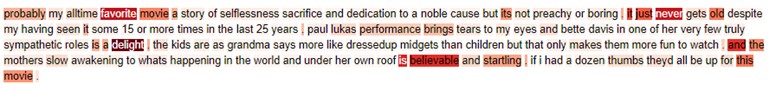
Figure 3 - Attention-Based token importance
We see that the word groups "favorite movie", "it just never gets old", "performance brings tears", or "it is believable and startling" stand out. This explains well why the algorithm evaluated the review as positive and what was the semantic field at the root of this prediction.
Next step
We will show in a future article how attention coefficients are useful for generating counterfactual examples to explain the model prediction.
References
[1] VASWANI, Ashish, SHAZEER, Noam, PARMAR, Niki, et al. Attention is all you need. Advances in neural information processing systems, 2017, vol. 30.
[2] SANH, Victor, DEBUT, Lysandre, CHAUMOND, Julien, et al. DistilBERT, a distilled version of BERT: smaller, faster, cheaper and lighter. arXiv preprint arXiv:1910.01108, 2019.
[3] Hugging face library https://huggingface.co/