Calibration tutorial
![]()
Note
Estimating the epidemiological parameters on real data is called *calibration*, in this tutorial we will see how pyepidemics can be used for such purpose. We will see how to calibrate a COVID19 model on French data
Developer import
%matplotlib inline
%load_ext autoreload
%autoreload 2

# Developer import
import sys
sys.path.append("../../")
On Google Colab
Uncomment the following line to install the library locally
# !pip install pyepidemics
Verify the library is correctly installed
import pyepidemics
Getting data
Some data helpers have been built in a scikit learn fashion to help you easily fetch data. For now it's only for French cases data, but feel free to contribute to add more data sources.
from pyepidemics.dataset import fetch_daily_case_france
We already have the compartments ready, cases have been also interpolated and smoothed to account for reporting errors
cases = fetch_daily_case_france()
cases.head()
cases[["D","R","H","ICU"]].plot(figsize = (15,4),title = "Real data France");

First COVID19 model without calibration
We will use a COVID19 differential equation model with a prodromal phase and 3 levels of symptoms. This model has been validated by epidemiologists and is similar to other researchers' model like the one from INSERM.
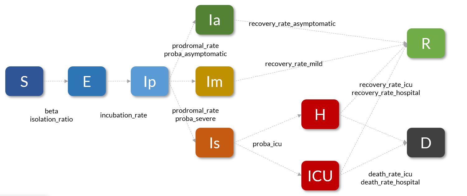
Most parameters have been initialized by default according to INSERM and Pasteur research paper, other parameters are as followed.
As shown in other tutorials we will simulate the French lockdown with a \beta going from beta_high to beta_low at the date 53 (First data is available for France on 2020-01-24 and lockdown started on 2020-03-17, ie 53 days later)
N = 67e6 # French population
beta_high = 0.9 # R0 around 3.3
beta_low = 0.16 # R0 around 0.6
beta = [beta_high,[beta_low],[53]] # We go from R0 around 3.6 to O.6 during lockdown starting at day 53
from pyepidemics.models import COVID19Prodromal

model = COVID19Prodromal(
    N = N,
    beta = beta,
    I0 = 5,
)
To tweak all other parameters you can see the help
help(model.__init__)
Let's make a prediction
states = model.solve(n_days = 200)
states[["H","ICU","D"]].show(plotly = False)

We will want to compare the curves to the real data, this can be done easily with the following functions
model.show_prediction(cases[["H","ICU","D"]])


The model is just ok, the peak and scale are not that far, but the global dynamics is not close enough to hope to use it for predictions. That's why we need calibration, we will iterate over the set of possible parameters to find a better fit.
We can also observe the reproduction factor R0, which is little low compared to estimates of around 3.3 by epidemiologists.
model.R0(0.9)
Calibrating the COVID19 model on France data
Preparing for calibration
To extend a model for calibration, we need to subclass the model to add a .reset() function explaining how to initialize a model with a tested set of parameters
N = 67e6

class CalibratedCOVID19(COVID19Prodromal):
    def __init__(self,params = None):
        if params is not None:
            self.reset(params)

    def reset(self,params):
        beta = [params["beta_high"],[params["beta_low"]],[53]]
        super().__init__(N = N ,beta = beta,**params)
        self.calibrated_params = params

model = CalibratedCOVID19()
We also need a space of parameters to test, those range are done accordingly to research papers on the topic for France data, it should be adapted to other situations.
Some parameters like probabilities at the hospital are not calibrated because we are quite confident in their literature values.
space = {
    "beta_low":(0.01,0.4),
    "beta_high":(0.6,1.5),
    "I0":(0,100),
    "recovery_rate_asymptomatic":(1/8,1/2),
    "recovery_rate_mild":(1/8,1/2),
    "death_rate_hospital":(0.006,0.02),
    "death_rate_icu":(0.006,0.02),
    "recovery_rate_icu":(0.02,0.08),
    "recovery_rate_hospital":(0.02,0.08),
}
Finally because we know the reproduction factor supposed value for COVID19 we can also pass a constraint callback to help the search of parameters. This constraint will augment the loss if the R0 is not in the intended range.
def constraint(model,loss):
    R0 = model.R0(model.calibrated_params["beta_high"])
    if R0 < 3 or R0 > 3.4:
        return loss*10
    else:
        return loss
Calibration with bayesian optimization
Once everything is setup you can use the calibration helper function. In a scikit learn fashion the function is simply called .fit()
Within this function, a bayesian optimization search process is run the same way you would look for the optimal hyperparameters in a Machine Learning problem. This is done with the Optuna library
We will fit on 3 epidemic curves : deaths (D), ICU and hospital (H) because the other data points such as number of confirmed cases are not reliable because of asymptomatic cases and testing policies. The loss function will be a composition of the RMSE loss for each curve.
We will run for n iterations, with an early stopping value is the best set of parameters has not changed for a while. You can try running for a longer period of time to see if you find better parameters.
model.fit(
    cases[["D","H","ICU"]],
    space,
    n = 200,
    early_stopping = 100,
#     constraint = constraint,
)
Visualizing the results
We can again compare the prediction with real data
model.show_prediction(cases[["H","ICU","D"]])


We can also better understand the internals of the optimization by visualizing the set of tested parameters in a parallel coordinates graph
model.opt.show_parallel_coordinates()
You can also estimate confidence interval by sampling among the tested parameters in the bayesian optimization
params_dist = model.opt.estimate_params_distributions(summary = True)
params_dist